0%

参考:https://networkx.github.io/documentation/stable/tutorial.html#adding-attributes-to-graphs-nodes-and-edges

引入networkx以及绘图所需的matplotlib。

1
2
import networkx as nx
import matplotlib.pyplot as plt
1
%matplotlib inline

1.图、点与边

生成空图,不包含

1
G = nx.Graph()

向图G中添加点。可一次只添加一个或直接添加列表。检索方式跟一维list类似。

1
2
3
4
5
6
G.add_node(1)
G.add_nodes_from([2,3])
G.nodes[1] # 检索获取点的方式1
G[1] # 检索获取点的方式2
print(G.nodes()) # 获取所有点的名称
print(G.nodes.data()) # 获取所有点的名称及相应的属性
[1, 2, 3]
[(1, {}), (2, {}), (3, {})]

此时可以显示G包含的点的数目。

1
G.number_of_nodes()
3

清除G的内容。

1
G.clear()

类似的方式可生成单个边或一系列的边。检索方式跟二维list类似。

1
2
3
4
5
6
G.add_edge('a','b')
G.add_edges_from((['c','d'],['e','f']))
print(G.number_of_nodes())# 显示当前节点数目
print(G.number_of_edges())# 显示当前边的数目
G.edges['a','b'] # 检索获取边的方式1
G['a']['b'] # 检索获取边的方式2
6
3


{}

文档中介绍,任意hasable的对象都可以作为点,常用的如:数字或字符。而边又可与任意object建立联系,G.add_edge(n1, n2, object=x)

一个Graph也可以从另一个Graph继承过来点或边。

1
2
3
H = nx.path_graph(10)
G.add_nodes_from(H)
G.add_edges_from(H.edges)

2.向图形、节点和边添加属性

除去图、点和边之间的包含以及连接的关系外,各个个体还可包含有自身相关的信息,例如名称、颜色或重量等等的属性。 属性的结构为:键/值(key/value),键应当是hasable的,也就是说属性是一个字典结构。属性默认为空,但是可以通过add_edge,add_node 进行修改。对于图G来说,也可以直接操作属性字典:G.graph,G.nodes,G.edges,于修改字典的操作相同。

图的属性

1
2
3
4
5
G = nx.Graph(day="Friday")
print(G.graph) # 显示属性 键/值
print(G.graph['day'])# 显示某个属性的值
G.graph['day']='Monday'
print(G.graph) # 显示属性 键/值
{'day': 'Friday'}
Friday
{'day': 'Monday'}

点的属性

1
2
3
4
5
G.add_node(1, time='5pm')
G.add_nodes_from([3], time='2pm')
print(G.nodes[1]) # 获取节点1的属性 注意用的是索引符号'[]'
G.nodes[1]['room'] = 714
G.nodes.data()
{'time': '5pm'}


NodeDataView({1: {'time': '5pm', 'room': 714}, 3: {'time': '2pm'}})

边的属性

特殊属性weight应该是数字,因为它被需要加权边缘的算法使用

1
2
3
4
5
G.add_edge(1, 2, weight=4.7 )
G.add_edges_from([(3, 4), (4, 5)], color='red')
G.add_edges_from([(1, 2, {'color': 'blue'}), (2, 3, {'weight': 8})])
G[1][2]['weight'] = 4.7
G.edges[3, 4]['weight'] = 4.2

3.访问相邻节点

1
2
3
4
5
FG = nx.Graph()
FG.add_weighted_edges_from([(1, 2, 0.125), (1, 3, 0.75), (2, 4, 1.2), (3, 4, 0.375)])
print(FG.adj.items())# 显示相邻的节点,无向图的情况下
print(list(FG.neighbors(1)))# 显示节点1的相邻节点的名称
print(list(FG.adj[1]))# 显示节点1的相邻节点的名称 与上一句作用相等
ItemsView(AdjacencyView({1: {2: {'weight': 0.125}, 3: {'weight': 0.75}}, 2: {1: {'weight': 0.125}, 4: {'weight': 1.2}}, 3: {1: {'weight': 0.75}, 4: {'weight': 0.375}}, 4: {2: {'weight': 1.2}, 3: {'weight': 0.375}}}))
[2, 3]
[2, 3]

4.绘图

参考文档中给出了draw函数的详细参数draw(G, pos=None, ax=None, **kwds)。其中pos的介绍如下: * pos (dictionary, optional) – A dictionary with nodes as keys and positions as values. If not specified a spring layout positioning will be computed. See networkx.drawing.layout for functions that compute node positions. 也就是说pos是一个字典结构,节点的名称作为key,坐标list作为value。

1
2
3
4
5
HTG = nx.Graph()
HTG.add_nodes_from([1,2,3])
HTG.add_edges_from(([1,2],[2,3],[3,1]))
pos={1:[0,1],2:[1,1],3:[2,2]}
nx.draw(HTG,pos=pos, with_labels=True, font_weight='bold')
png
png

5.有向图

DiGraph 类为有方向的边提供了额外的属性,例如DiGraph.out_edges(),DiGraph.in_degree(),DiGraph.predecessors(),DiGraph.successors(),等等。为使算法在处理不同类上更加便利,有方向版本的neighbors等价于successors()。同时degree表示in_degreeout_degree之和。这种处理有时可能感觉不是特别一致。

1
2
3
4
5
6
7
DG = nx.DiGraph()
DG.add_weighted_edges_from([(1, 2, 0.5), (3, 1, 0.75)])
print(DG.out_degree(1, weight='weight'))
print(DG.degree(1, weight='weight'))
print(list(DG.successors(1)))
print(list(DG.neighbors(1)))
nx.draw(DG, with_labels=True, font_weight='bold')
0.5
1.25
[2]
[2]
png
png

有向图可以转换为无向图。可利用Graph.to_undirected()Graph()

1
2
3
4
H1 = nx.Graph.to_undirected(DG)
nx.draw(H1, with_labels=True, font_weight='bold')
H2 = nx.Graph(DG)
nx.draw(H2, with_labels=True, font_weight='bold')
png
png

6.点与线分别设置样式

1
2
3
4
5
6
7
8
9
10
11
12
13
14
15
16
17
18
DG = nx.DiGraph()
DG.add_weighted_edges_from([(1, 2, 0.5), (3, 1, 0.75)])
# nx.draw(DG, with_labels=True, font_weight='bold') # 将nx.draw替换为nx.draw_networkx_nodes和nx.draw_networkx_edges
# 点的样式
options = {
'node_color': 'blue',
'node_size': 50,
'alpha':1,
}
nx.draw_networkx_nodes(DG,pos=pos,**options)
# 边的样式
options = {
'line_color': 'grey',
'linewidths': 0,
'width': 2,
'alpha':0.5,
}
nx.draw_networkx_edges(DG,pos=pos,**options)
[<matplotlib.patches.FancyArrowPatch at 0x25e4dbc6948>,
 <matplotlib.patches.FancyArrowPatch at 0x25e4dbca1c8>]
png
png

7.遍历边的属性

根据参考文档中networkx.Graph.edges的说明。该函数主要有一个data参数,当设置为True的时候返回(起点,终点,data字典),当为False的时候返回(起点,终点)。

1
2
3
4
5
6
7
8
9
10
DG = nx.DiGraph()
DG.add_weighted_edges_from([(1, 2, 0.5), (3, 1, 0.75)])
for u,v,d in DG.edges(data=True):
print(d['weight'])
edges_list = [(u, v, d) for (u, v, d) in DG.edges(data=True)]
print(edges_list)
print(edges_list[0][2]['weight'])
edges = list(DG.edges(data=True))
print(edges)
print(edges[0][2]['weight'])
0.5
0.75
[(1, 2, {'weight': 0.5}), (3, 1, {'weight': 0.75})]
0.5
[(1, 2, {'weight': 0.5}), (3, 1, {'weight': 0.75})]
0.5

问题描述:

此问题是我在更新Hexo后发现的。利用hexo-asset-image并无法显示图片。查看网上资料,有的说是Hexo 3版本后的兼容性问题,但大多都是语焉不详的粘贴复制,并不能解决问题。而经过一番ballache的折腾后,发现问题在于hexo-asset-image的源码中,下面给出具体的解决方案。 ## 解决方案: 首先贴出Hexo及使用的库的详细版本,此解决方案至少针对当前环境可用,大家可自行修改环境。 package.json文件内容:

1
2
3
4
5
6
7
8
9
10
11
12
13
14
15
16
17
18
19
20
21
22
23
24
25
26
{
"name": "hexo-site",
"version": "0.0.0",
"private": true,
"hexo": {
"version": "4.2.1"
},
"dependencies": {
"hexo": "^4.2.1",
"hexo-asset-image": "^1.0.0", 这个需要安装,同时设置_config.yml文件中的hexo-asset-folder: true
"hexo-asset-link": "^2.0.1",
"hexo-deployer-git": "^2.1.0",
"hexo-generator-archive": "^1.0.0",
"hexo-generator-category": "^1.0.0",
"hexo-generator-index": "^1.0.0",
"hexo-generator-tag": "^1.0.0",
"hexo-image-link": "0.0.3",
"hexo-inject": "^1.0.0",
"hexo-renderer-ejs": "^1.0.0",
"hexo-renderer-kramed": "^0.1.4",
"hexo-renderer-pandoc": "^0.3.0",
"hexo-renderer-pug": "^1.0.0",
"hexo-renderer-stylus": "^1.1.0",
"hexo-server": "^1.0.0"
}
}
打开_modules-asset-image.js文件。修改24和57行。
1
2
3
4
5
6
7
8
9
10
11
12
13
14
15
16
17
18
19
20
21
22
23
24
25
26
27
28
29
30
31
32
33
34
35
36
37
38
39
40
41
42
43
44
45
46
47
48
49
50
51
52
53
54
55
56
57
58
59
60
61
62
63
64
65
66
67
68
69
70
71
'use strict';
var cheerio = require('cheerio');

// http://stackoverflow.com/questions/14480345/how-to-get-the-nth-occurrence-in-a-string
function getPosition(str, m, i) {
return str.split(m, i).join(m).length;
}

hexo.extend.filter.register('after_post_render', function(data){
var config = hexo.config;
if(config.post_asset_folder){
var link = data.permalink;
var beginPos = getPosition(link, '/', 3) + 1;
var appendLink = '';
// In hexo 3.1.1, the permalink of "about" page is like ".../about/index.html".
// if not with index.html endpos = link.lastIndexOf('.') + 1 support hexo-abbrlink
if(/.*\/index\.html$/.test(link)) {
// when permalink is end with index.html, for example 2019/02/20/xxtitle/index.html
// image in xxtitle/ will go to xxtitle/index/
appendLink = 'index/';
var endPos = link.lastIndexOf('/');
}
else {
//var endPos = link.lastIndexOf('.'); 修改位置1,修改为var endPos = link.length-1;
var endPos = link.length-1;
}
link = link.substring(beginPos, endPos) + '/' + appendLink;

var toprocess = ['excerpt', 'more', 'content'];
for(var i = 0; i < toprocess.length; i++){
var key = toprocess[i];

var $ = cheerio.load(data[key], {
ignoreWhitespace: false,
xmlMode: false,
lowerCaseTags: false,
decodeEntities: false
});

$('img').each(function(){
if ($(this).attr('src')){
// For windows style path, we replace '\' to '/'.
var src = $(this).attr('src').replace('\\', '/');
if(!(/http[s]*.*|\/\/.*/.test(src)
|| /^\s+\//.test(src)
|| /^\s*\/uploads|images\//.test(src))) {
// For "about" page, the first part of "src" can't be removed.
// In addition, to support multi-level local directory.
var linkArray = link.split('/').filter(function(elem){
return elem != '';
});
var srcArray = src.split('/').filter(function(elem){
return elem != '' && elem != '.';
});
if(srcArray.length > 1)
srcArray.shift();
//src = srcArray.join('/'); 修改位置1,修改为src = '/'+ srcArray[srcArray.length-1];
src = '/'+ srcArray[srcArray.length-1];
$(this).attr('src', config.root + link + src);
console.info&&console.info("update link as:-->"+config.root + link + src);

}
}else{
console.info&&console.info("no src attr, skipped...");
console.info&&console.info($(this));
}
});
data[key] = $.html();
}
}
});
此时不论用markdown语法还是asset_img语法都可以显示。
1
2
![图1](Image1.png)
{% asset_img Image1.png 图1 %}
修改_config.yml文件。需要修改两个地方:
1
2
3
4
5
6
7
8
修改处1,修改为true后,每次new blog的时候都会在md文件的目录下生成同名的blog文件夹,然后图片都放到该文件夹里面就可以了,这个百度搜搜就都有更详细的介绍。
post_asset_folder: true

修改处2,把url改成你的github的网址,这个用github做blog仓的都知道是啥地址。
# URL
## If your site is put in a subdirectory, set url as 'http://yoursite.com/child' and root as '/child/'
url: https://你的名字.github.io
root: /
这样就OK了。

问题解决过程

1.首先百度问题关键字,解决方案统统无效,但至少在这个阶段更新了Hexo版本...... 2.chrome中F12,在开发者模式下研究无法显示的图片的元素。 
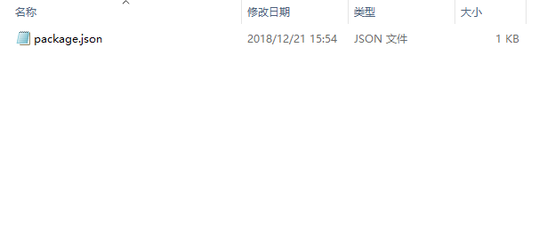
发现路径不对,图片中的可能跟你的不一样,但总而言之就是地址有问题。 3.在hexo-asset-image的github页面中的issues里发现有人提出同样的问题,然后看到说是源码的地址处理的问题。虽然开发者发现了问题,但是npm安装的依旧有问题。于是乎最简单的解决方法就是自己改index.js的源码里地址生成的部分。

参考资料:https://www.gams.com/latest/docs/API_PY_TUTORIAL.html

引入必要模块

1
2
3
4
5
# gams模块
from gams import *
# 常用python自带模块
import os
import sys

多Gams系统下的选择

1
2
3
4
5
# 多gams版本环境下,shell中运行py文件时可选择与default不同的gams版本运行,用以下语句进行控制
if len(sys.argv) > 1:
ws = GamsWorkspace(system_directory = sys.argv[1])
else:
ws = GamsWorkspace()

数据结构

1
2
3
4
5
6
7
8
9
10
11
plants = [ "Seattle", "San-Diego" ]
markets = [ "New-York", "Chicago", "Topeka" ]
capacity = { "Seattle": 350.0, "San-Diego": 600.0 }
demand = { "New-York": 325.0, "Chicago": 300.0, "Topeka": 275.0 }
distance = { ("Seattle", "New-York") : 2.5,
("Seattle", "Chicago") : 1.7,
("Seattle", "Topeka") : 1.8,
("San-Diego", "New-York") : 2.5,
("San-Diego", "Chicago") : 1.8,
("San-Diego", "Topeka") : 1.4
}

在python代码中,gams中的set用list表示(如plants或markets),gams中的parameter则用dic表示(如demand或capacity)。

  • GamsDatabase 是python数据与gams进行交换的中转变量。
    1
    2
    3
    4
    5
    6
    7
    8
    9
    10
    11
    12
    13
    14
    15
    # 创建新的GamsDatabase实例
    db = ws.add_database()

    # 往GamsDatabase中增添一维集合 'i' ,文本'canning plants'进行解释说明
    i = db.add_set("i", 1, "canning plants")
    for p in plants:
    i.add_record(p)

    # 增加定义域为 i' 的参数 'a'
    a = db.add_parameter_dc("a", [i], "capacity of plant i in cases")
    for p in plants:
    a.add_record(p).value = capacity[p]

    # 在项目空间的工作目录中,将GamsDatabase输出到名为'data.gdx' 的GDX (GAMS Data eXchange)文件
    db.export("data.gdx")
    GDX文件可在gams studio中打开并显示。同时可使用gdx-pandas将GDX转化为DataFrame结构。

运行gms文件

1
2
3
# 注意文件要有路径
t1 = ws.add_job_from_file(路径/"你的文件.gms")
t1.run()

可在运行前进行option设置。

1
2
3
4
# 将xpress设置为默认solver
opt = ws.add_options()
opt.all_model_types = "xpress"
t1.run(opt)

输出运行日志

1
2
3
4
5
6
7
8
9
10
path=os.getcwd()# 获取当前路径
file = open(r"%s\xpress.opt"%(path), "w")# 打开一个xpress.opt设置文件
file.write("algorithm=barrier")# 在设置文件中进行算法设置
file.close()
opt.optfile = 1# 改设置令solver运行前读取opt设置
# 运行日志输出到本地文件xpress.log中
with open("xpress.log", "w") as log:
t1.run(opt, output=log)
# 如果想输出到显示屏上
t1.run(opt, output=sys.stdout)

输出运行结果

以如下小例子为例。gms代码如下

1
2
3
4
5
6
7
8
9
10
11
12
13
14
15
16
17
18
19
20
21
22
23
24
25
Set
i /i1*i3/;

parameter
C(i)
/
i1 1
i2 2
i3 3
/;
free variable
x(i)
Z;

equations
objective
cons;

objective.. Z =e= sum(i,C(i)*x(i));
cons(i).. x(i) =g= 0;

Model MyModel /all/;

solve MyModel using lp minimizing Z;
display x.l, x.m;
pyton代码
1
2
3
4
path=os.getcwd()
t1 = ws.add_job_from_file(r"%s\test.gms"%(path))
for rec in t1.out_db.get_symbol("x"):
print("x(" + rec.keys[0] + "): level=" + str(rec.level) + " marginal=" + str(rec.marginal))
其中t1.out_db是GamsDatabase实例,也就可以输出到GDX文件中,然后用gams studio打开显示结果。

模型与数据分离(transport2.py为例)

代码中首先定义的数据函数,返回遵循gams语法规则的相关输入数据的定义。

1
2
3
4
5
6
7
8
9
10
11
12
13
14
15
16
17
18
19
20
21
22
23
def get_data_text():
return '''
Sets
i canning plants / seattle, san-diego /
j markets / new-york, chicago, topeka / ;

Parameters

a(i) capacity of plant i in cases
/ seattle 350
san-diego 600 /

b(j) demand at market j in cases
/ new-york 325
chicago 300
topeka 275 / ;

Table d(i,j) distance in thousands of miles
new-york chicago topeka
seattle 2.5 1.7 1.8
san-diego 2.5 1.8 1.4 ;

Scalar f freight in dollars per case per thousand miles /90/ ; '''
接着又定义了模型函数,返回遵循gams语法规则的模型文本。其中只给出了集合及参数的声明,而未给出具体数值。
1
2
3
4
5
6
7
8
9
10
11
12
13
14
15
16
17
18
19
20
21
22
23
24
25
26
27
28
29
30
31
32
33
34
35
36
37
38
39
40
41
def get_model_text():
return '''
Sets
i canning plants
j markets

Parameters
a(i) capacity of plant i in cases
b(j) demand at market j in cases
d(i,j) distance in thousands of miles
Scalar f freight in dollars per case per thousand miles;

$if not set incname $abort 'no include file name for data file provided'
$include %incname%

Parameter c(i,j) transport cost in thousands of dollars per case ;

c(i,j) = f * d(i,j) / 1000 ;

Variables
x(i,j) shipment quantities in cases
z total transportation costs in thousands of dollars ;

Positive Variable x ;

Equations
cost define objective function
supply(i) observe supply limit at plant i
demand(j) satisfy demand at market j ;

cost .. z =e= sum((i,j), c(i,j)*x(i,j)) ;

supply(i) .. sum(j, x(i,j)) =l= a(i) ;

demand(j) .. sum(i, x(i,j)) =g= b(j) ;

Model transport /all/ ;

Solve transport using lp minimizing z ;

Display x.l, x.m ; '''
其中以下两句判断是否有名为incname的option被引入。经测试,可放置在get_model_text()的return文本中的任意位置。
1
2
$if not set incname $abort 'no include file name for data file provided'
$include %incname%
python执行代码如下:
1
2
3
4
5
6
7
8
9
10
11
12
13
14
15
16
17
18
19
20
21
if __name__ == "__main__":
if len(sys.argv) > 1:
ws = GamsWorkspace(system_directory = sys.argv[1])
else:
ws = GamsWorkspace()

# 将文本输出到tdata.gms文件中 注意这里的路径为ws.working_directory,最好不要自己该路径
file = open(os.path.join(ws.working_directory, "tdata.gms"), "w")
file.write(get_data_text())
file.close()

# 将字符串定义的模型添加到job中
t2 = ws.add_job_from_string(get_model_text())
# 添加设置
opt = ws.add_options()
# 定义名为“incnmae”的option(可随意选择名称,但需要与上面$if...中的一致)。“tdata”是刚输出的data_text文件,也可写为"tdata.gms"或“路径/tdata.gms”
opt.defines["incname"] = "tdata"
# 执行代码并输出
t2.run(opt)
for rec in t2.out_db["x"]:
print("x(" + rec.key(0) + "," + rec.key(1) + "): level=" + str(rec.level) + " marginal=" + str(rec.marginal))

尝试改动,将变量定义放到get_data_text中,然后又定义了get_variable_set函数固定x的值。在get_model_text中多加一个include。在运行代码中添加了option。

1
2
3
4
5
6
7
8
9
10
11
12
13
14
15
16
17
18
19
20
21
22
23
24
25
26
27
28
29
30
31
32
33
34
35
36
37
38
39
40
41
42
43
44
45
46
47
48
49
50
51
52
53
54
55
56
57
58
59
60
61
62
63
64
65
66
67
68
69
70
71
72
73
74
75
76
77
78
79
80
81
82
83
84
85
86
87
88
89
90
91
92
93
94
95
96
97
98
def get_data_text():
return '''
Sets
i canning plants / seattle, san-diego /
j markets / new-york, chicago, topeka / ;

Parameters

a(i) capacity of plant i in cases
/ seattle 350
san-diego 600 /

b(j) demand at market j in cases
/ new-york 325
chicago 300
topeka 275 / ;

Table d(i,j) distance in thousands of miles
new-york chicago topeka
seattle 2.5 1.7 1.8
san-diego 2.5 1.8 1.4 ;

Scalar f freight in dollars per case per thousand miles /90/ ;

Variables
x(i,j) shipment quantities in cases
z total transportation costs in thousands of dollars ;

Positive Variable x ;

'''

def get_variable_set():
return '''
x.fx('seattle','new-york')=25;
'''


def get_model_text():
return '''
$if not set incname1 $abort 'no include file name for data file provided'
$if not set incname2 $abort 'no include file name for data file provided'
$include %incname1%
$include %incname2%
Sets
i canning plants
j markets

Parameters
a(i) capacity of plant i in cases
b(j) demand at market j in cases
d(i,j) distance in thousands of miles
Scalar f freight in dollars per case per thousand miles;

Parameter c(i,j) transport cost in thousands of dollars per case ;

c(i,j) = f * d(i,j) / 1000 ;


Equations
cost define objective function
supply(i) observe supply limit at plant i
demand(j) satisfy demand at market j ;

cost .. z =e= sum((i,j), c(i,j)*x(i,j)) ;

supply(i) .. sum(j, x(i,j)) =l= a(i) ;

demand(j) .. sum(i, x(i,j)) =g= b(j) ;

Model transport /all/ ;

Solve transport using lp minimizing z ;

Display x.l, x.m ; '''

if __name__ == "__main__":
if len(sys.argv) > 1:
ws = GamsWorkspace(system_directory = sys.argv[1])
else:
ws = GamsWorkspace()

file = open(os.path.join(ws.working_directory, "tdata1.gms"), "w")
file.write(get_data_text())
file.close()

file = open(os.path.join(ws.working_directory, "tdata2.gms"), "w")
file.write(get_variable_set())
file.close()

t2 = ws.add_job_from_string(get_model_text())
opt = ws.add_options()
opt.defines["incname1"] = "tdata1.gms"
opt.defines["incname2"] = "tdata2.gms"
t2.run(opt)
for rec in t2.out_db["x"]:
print("x(" + rec.key(0) + "," + rec.key(1) + "): level=" + str(rec.level) + " marginal=" + str(rec.marginal))

利用GamsModifier修改模型实例的parameter和variable

首先需要了解 GamsCheckpoint ,其作用是捕捉GamsJob的状态。详细解释如下:

1
2
3
4
5
6
# 定义一个checkpoint
cp = ws.add_checkpoint()
# 利用string定义一个GamsJob t5 但string中不含有solve语句
t5 = ws.add_job_from_string(get_model_text())
# 利用checkpoint捕捉及控制GamsJob
t5.run(checkpoint=cp)
其中get_model_text()具体如下,注意没有像前面的代码中一样包含“ Solve transport using lp minimizing z ;”的语句。
1
2
3
4
5
6
7
8
9
10
11
12
13
14
15
16
17
18
19
20
21
22
23
24
25
26
27
28
29
30
31
32
33
34
35
36
37
38
39
40
41
42
43
44
45
46
47
48
def get_model_text():
return '''
Sets
i canning plants / seattle, san-diego /
j markets / new-york, chicago, topeka / ;

Parameters

a(i) capacity of plant i in cases
/ seattle 350
san-diego 600 /

b(j) demand at market j in cases
/ new-york 325
chicago 300
topeka 275 / ;

Table d(i,j) distance in thousands of miles
new-york chicago topeka
seattle 2.5 1.7 1.8
san-diego 2.5 1.8 1.4 ;

Scalar f freight in dollars per case per thousand miles /90/ ;
Scalar bmult demand multiplier /1/;

Parameter c(i,j) transport cost in thousands of dollars per case ;

c(i,j) = f * d(i,j) / 1000 ;

Variables
x(i,j) shipment quantities in cases
z total transportation costs in thousands of dollars ;

Positive Variable x ;

Equations
cost define objective function
supply(i) observe supply limit at plant i
demand(j) satisfy demand at market j ;

cost .. z =e= sum((i,j), c(i,j)*x(i,j)) ;

supply(i) .. sum(j, x(i,j)) =l= a(i) ;

demand(j) .. sum(i, x(i,j)) =g= bmult*b(j) ;

Model transport /all/ ;
Scalar ms 'model status', ss 'solve status'; '''
利用checkpoint可以实现变换输入,进行多次Job运算,得到相应的结果。
1
2
3
4
5
6
7
8
9
10
11
12
13
14
15
16
17
18
19
20
21
22
23
24
25
if __name__ == "__main__":
if len(sys.argv) > 1:
ws = GamsWorkspace(system_directory = sys.argv[1])
else:
ws = GamsWorkspace()

cp = ws.add_checkpoint()

# initialize a GAMSCheckpoint by running a GAMSJob
t5 = ws.add_job_from_string(get_model_text())
t5.run(checkpoint=cp)

# 定义了bmultlist的不同取值
bmultlist = [ 0.6, 0.7, 0.8, 0.9, 1.0, 1.1, 1.2, 1.3 ]

# create a new GAMSJob that is initialized from the GAMSCheckpoint
for b in bmultlist:
# 针对不同的bmult取值生成具有不同输入的Job t5,并添加solve 语句。checkpoint cp 也作为参数输入,个人理解是新输入的语句+cp拼合成完整包含不同参数和求解语句的模型。
t5 = ws.add_job_from_string("bmult=" + str(b) + "; solve transport min z use lp; ms=transport.modelstat; ss=transport.solvestat;", cp)
# 执行Job并输出结果,结果储存在GamsDatabase类型变量t5.out_db中。
t5.run()
print("Scenario bmult=" + str(b) + ":")
print(" Modelstatus: " + str(t5.out_db["ms"].find_record().value))
print(" Solvestatus: " + str(t5.out_db["ss"].find_record().value))
print(" Obj: " + str(t5.out_db["z"].find_record().level))
接着介绍如何使用checkpoint创建GamsModelInstance。个人感觉GamsModelInstance的作用跟Job是一样的,都是可以用来进行模型运算,输出结果。同时可以实现变动参数和变动变量下的模型输出。
1
2
3
4
5
6
7
8
9
10
11
12
13
14
15
16
17
18
19
20
21
22
23
24
25
26
27
28
29
30
31
32
33
34
35
36
37
38
39
40
41
42
43
44
45
46
47
48
49
50
51
52
53
54
55
56
57
58
59
60
61
62
63
64
65
66
67
68
69
70
71
72
73
74
75
76
77
if __name__ == "__main__":
if len(sys.argv) > 1:
ws = GamsWorkspace(system_directory = sys.argv[1])
else:
ws = GamsWorkspace()
# 生成checkpoint
cp = ws.add_checkpoint()

# initialize a GAMSCheckpoint by running a GAMSJob
t7 = ws.add_job_from_string(get_model_text())# 生成包含模型部分的job,但不包含solve语句
t7.run(checkpoint=cp)# 运行job,将状态传递给checkpoint,大约意味着checkpoint获得了模型信息,包括数据和公式

# 下面部分是实现每次运行都可以有不同的参数设置
# create a GAMSModelInstance and solve it multiple times with different scalar bmult
mi = cp.add_modelinstance()# 生成模型实例
bmult = mi.sync_db.add_parameter("bmult", 0, "demand multiplier")# 向改实例中添加参数,函数参数2:0表示维度dim为0 可输出到gdx中查看,此时bmult还是空值,结果为下图1
opt = ws.add_options()# 向工作空间中添加option,这个是公用的
opt.all_model_types = "cplexd"# 设定求解器
# opt.all_model_types = "gurobi" 文档中给出的另一个实例

# instantiate the GAMSModelInstance and pass a model definition and GAMSModifier to declare bmult mutable
mi.instantiate("transport use lp min z", GamsModifier(bmult), opt)# 参数1增添了solve语句;参数2表示参数bmult在运行时是可变的,而其他参数等式不变;参数3表示使用上面给的设置;此时输出到gdx可见模型参数已经随opt传入,bmult依旧是空值,具体见图2

bmult.add_record().value = 1.0# 给可变参数bmult添加初始值 此时输出gdx可见bmult已经有数值,见图3
bmultlist = [ 0.6, 0.7, 0.8, 0.9, 1.0, 1.1, 1.2, 1.3 ]

print("Scenario bmult=" + str(mi.sync_db['bmult'].find_record().value))# 可显示当前场景下bmult的数值 下面语句一样的效果
print("Scenario bmult=" + str(mi.sync_db.get_parameter('bmult').find_record().value))# 可显示当前场景下bmult的数值


for b in bmultlist:
bmult.first_record().value = b# 求解前给bmult赋不同值
mi.solve()# 模型求解
print("Scenario bmult=" + str(b) + ":")
print(" Modelstatus: " + str(mi.model_status))
print(" Solvestatus: " + str(mi.solver_status))
print(" Obj: " + str(mi.sync_db.get_variable("z").find_record().level))

#下面部分是实现运行时有不同的变量设置
# create a GAMSModelInstance and solve it with single links in the network blocked
mi = cp.add_modelinstance()# 生成实例
x = mi.sync_db.add_variable("x", 2, VarType.Positive)# 向实例中添加变量,函数参数2:“2”表示维度是2,函数参数3:VarType.Positive表示变量为正实数
xup = mi.sync_db.add_parameter("xup", 2, "upper bound on x")
# 此时输出到gdx,可见变量x和参数xup都还没哟具体数值。见图4

# instantiate the GAMSModelInstance and pass a model definition and GAMSModifier to declare upper bound of X mutable
mi.instantiate("transport use lp min z", GamsModifier(x, UpdateAction.Upper, xup))# 生成实例。GamsModifier用来制定x是的某些属性是可更改的,参数UpdateAction.Upper即表示改属性(具体表示x的上界upper bound可变)。文档给出三种可变属性:
lower bound, upper bound or level。UpdateAction类的详细信息科参见文档,包含Upper、Lower 、Fixed、Primal和Dual等五种选择。参数xup为对应的属性更换的数值。虽然没有像上面参数的例子添加opt参数,但输出的gdx中已经包含模型的集合等数据。见图5。
mi.solve()

for i in t7.out_db["i"]:
for j in t7.out_db["j"]:
xup.clear()# 清除xup设置
xup.add_record((i.key(0),j.key(0))).value = 0 # 为某一link设置上界为零,见图6
mi.solve()
print("Scenario link blocked: " + i.key(0) + " - " + j.key(0))
print(" Modelstatus: " + str(mi.model_status))
print(" Solvestatus: " + str(mi.solver_status))
print(" Obj: " + str(mi.sync_db["z"].find_record().level))

# 尝试使用。目标是固定某link必须使用,经测试成功。
mi = cp.add_modelinstance()
x = mi.sync_db.add_variable("x", 2, VarType.Positive)
xlevel = mi.sync_db.add_parameter("xlevel", 2, "fixed value of x")
mi.instantiate("transport use lp min z", GamsModifier(x, UpdateAction.Fixed, xlevel))# 令某link的x固定为xlevel=1
for i in t7.out_db["i"]:_config.yml
for j in t7.out_db["j"]:
xlevel.clear()
xlevel.add_record((i.key(0), j.key(0))).value = 1
# mi.solve()
path = os.getcwd()
mi.sync_db.export(r"%s\d.gdx" % (path))
mi.solve()
print("Scenario link forced: " + i.key(0) + " - " + j.key(0))
print(" Modelstatus: " + str(mi.model_status))
print(" Solvestatus: " + str(mi.solver_status))
print(" Obj: " + str(mi.sync_db["z"].find_record().level))
图1: 图2: 图3: 图4: 图5: 图6:

  • 有时需要从gms文件加载Job,但如果不特别设置,ws的working_directory是一个临时文件夹,可能找不到gms文件。在 https://forum.gamsworld.org/viewtopic.php?t=10228 给出了详细的解释。解决方案是:

    1
    ws = GamsWorkspace(working_directory=".")

  • 有时需要修改多个参数,这时就需要修改instantiate函数的第二个参数,改单一GamsModifier为跑list

    1
    mi.instantiate("transport use lp min z", [GamsModifier(g1),GamsModifier(g2)...,GamsModifier(gn)], opt)
    参考说明文档:https://www.gams.com/latest/docs/apis/java/classcom_1_1gams_1_1api_1_1GAMSModelInstance.html#af6afd2f81e9e3ca7ee4656ee467afe49

  • 有时需要修改一个parameters,也就是一个list的初始值。这时比较麻烦,因为该参数需要set作为add函数的第二个输入变量,然而这个set无法一开始就在sync_db中定义。于是需要一个迂回的操作,具体如下:

1
2
3
4
5
6
7
8
9
10
11
12
# 得到集合 用作add_parameter的第二个参数 此时record locked无法增加修改
Si=mi.sync_db.add_set("Si",1,"集合")
S0 = mi.sync_db.add_parameter_dc("S0", [Si], "需要修改的parameters")
# set 不允许作为GamsModifier。instantiate后就可以修改record
mi.instantiate("problem using mip max Z", [其他的GamsModifier...,GamsModifier(S0)])

# 为了能修改S0 即使gms文件中已经有Si的定义 但在这里还需要定义一遍
for s in 给出的Set:#给出的Set 就是一个list 如['i1','i2',...,'in']
Si.add_record(s)
# 给S0赋初始值
for s in S0的索引:
S0.add_record(s).value = 具体要赋予的初始值数值

编辑 themes/next/layout/_macro/sidebar.swig 文件
1
2
3
4
5
<div id="music_player">
{% if theme.background_music %}
<iframe width="560" height="315" src="{{theme.background_music}}" frameborder="0" allow="accelerometer; autoplay; encrypted-media; gyroscope; picture-in-picture" allowfullscreen></iframe>
{% endif %}
</div>
### 在 themes/next/_config.yml 配置文件中添加歌单地址配置
1
2
# background music
background_music: https://www.youtube.com/embed/_KesJL5EVjg

也可以直接将"iframe"文本整个粘贴到sidebar.swig 文件中

1
2
3
<div id="music_player">
<iframe width="560" height="315" src="https://www.youtube.com/embed/_KesJL5EVjg" frameborder="0" allow="accelerometer; autoplay; encrypted-media; gyroscope; picture-in-picture" allowfullscreen></iframe>
</div>

简介

GMAS的输出包含以下几部分: 1. 编译结果 编译结果包含输入文件的打印,可能的错误提示以及GMAS对象和交叉引用图列表。 2. 执行结果 执行结果包含展示声明的结果和可能的执行错误提示。 3. 模型生成 该结果在模型生成过程给出,包含等式和变量列表以及模型统计和可可能的生成执行时的错误提示。 4. 解 外部求解器程序处理模型时生成的解报告包括:求解总结,求解器的报告,解列表以及报告总结。 5. 解后输出 输出的最后部分包括最终执行总结和文件总结。

模型示例

1
2
3
4
5
6
7
8
9
10
11
12
13
14
15
16
17
18
19
20
21
22
23
24
25
26
27
28
29
30
31
32
33
34
35
36
37
38
39
40
41
42
43
44
45
46
47
48
49
50
51
$Title A Quadratic Programming Model for Portfolio Analysis (ALAN,SEQ=124a)

$onsymlist onsymxref onuellist onuelxref

$Ontext
This is a mini mean-variance portfolio selection problem described in
'GAMS/MINOS:Three examples' by Alan S. Manne, Department of Operations
Research, Stanford University, May 1986.
$Offtext

* This model has been modified for use in the documentation

Set i securities /hardware, software, show-biz, t-bills/;
alias (i,j);

Scalar target target mean annual return on portfolio % /10/,
lowyield yield of lowest yielding security,
highrisk variance of highest security risk ;

Parameters mean(i) mean annual returns on individual securities (%)
/ hardware 8
software 9
show-biz 12
t-bills 7 /

Table v(i,j) variance-covariance array (%-squared annual return)
hardware software show-biz t-bills
hardware 4 3 -1 0
software 3 6 1 0
show-biz -1 1 10 0
t-bills 0 0 0 0 ;

lowyield = smin(i, mean(i)) ;
highrisk = smax(i, v(i,i)) ;
display lowyield, highrisk ;

Variables x(i) fraction of portfolio invested in asset i
variance variance of portfolio
Positive Variable x;

Equations fsum fractions must add to 1.0
dmean definition of mean return on portfolio
dvar definition of variance;

fsum.. sum(i, x(i)) =e= 1.0;
dmean.. sum(i, mean(i)*x(i)) =e= target;
dvar.. sum(i, x(i)*sum(j,v(i,j)*x(j))) =e= variance;

Model portfolio / fsum, dmean, dvar / ;
Solve portfolio using nlp minimizing variance;
display x.l, variance.l;

1.编译输出

该结果在程序初始检查时生成。包括:输入文件的打印,符号引用图,符号清单图,特殊元素清单图和包含的文件总结。 ## 1.1 输入文件的打印 基本就是把输入的模型文本重新打印一遍。

1
2
3
4
5
6
7
8
9
10
A Quadratic Programming Model for Portfolio Analysis (ALAN,SEQ=124a)
C o m p i l a t i o n

2
4
This is a mini mean-variance portfolio selection problem described in
'GAMS/MINOS:Three examples' by Alan S. Manne, Department of Operations
Research, Stanford University, May 1986.
10
11 * This model has been modified for use in the documentation
1
2
3
4
5
6
7
8
9
10
11
12
13
14
15
16
17
18
19
20
21
22
23
24
25
26
27
28
29
30
31
32
33
34
35
36
37
38
39
40
12
13 Set i securities /hardware, software, show-biz, t-bills/;
14 alias (i,j);
15
16 Scalar target target mean annual return on portfolio % /10/,
17 lowyield yield of lowest yielding security,
18 highrisk variance of highest security risk ;
19
20 Parameters mean(i) mean annual returns on individual securities (%)
21 / hardware 8
22 software 9
23 show-biz 12
24 t-bills 7 / ;
25
26 Table v(i,j) variance-covariance array (%-squared annual return)
27 hardware software show-biz t-bills
28 hardware 4 3 -1 0
29 software 3 6 1 0
30 show-biz -1 1 10 0
31 t-bills 0 0 0 0 ;
32
33 lowyield = smin(i, mean(i)) ;
34 highrisk = smax(i, v(i,i)) ;
35 display lowyield, highrisk ;
36
37 Variables x(i) fraction of portfolio invested in asset i
38 variance variance of portfolio ;
39 Positive Variable x ;
40
41 Equations fsum fractions must add to 1.0
42 dmean definition of mean return on portfolio
43 dvar definition of variance;
44
45 fsum.. sum(i, x(i)) =e= 1.0;
46 dmean.. sum(i, mean(i)*x(i)) =e= target;
47 dvar.. sum(i, x(i)*sum(j,v(i,j)*x(j))) =e= variance;
48
49 Model portfolio / fsum, dmean, dvar / ;
50 Solve portfolio using nlp minimizing variance;
51 display x.l, variance.l;

1.2 符号引用图

1
2
3
4
5
6
7
8
9
10
11
12
13
14
15
16
17
18
19
Symbol Listing


SYMBOL TYPE REFERENCES

dmean EQU declared 42 defined 46 impl-asn 50 ref 49
dvar EQU declared 43 defined 47 impl-asn 50 ref 49
fsum EQU declared 41 defined 45 impl-asn 50 ref 49
highrisk PARAM declared 18 assigned 34 ref 35
i SET declared 13 defined 13 ref 14 20 26 33 2*34
37 45 2*46 2*47 control 33 34 45 46 47
j SET declared 14 ref 26 2*47 control 47
lowyield PARAM declared 17 assigned 33 ref 35
mean PARAM declared 20 defined 21 ref 33 46
portfolio MODEL declared 49 defined 49 impl-asn 50 ref 50
target PARAM declared 16 defined 16 ref 46
v PARAM declared 26 defined 26 ref 34 47
variance VAR declared 38 impl-asn 50 ref 47 50 51
x VAR declared 37 impl-asn 50 ref 39 45 46 2*47 51

头两列给出了符号的名字和类型。数据类型和简写如下:

Shorthand Symbol GAMS Data Type
ACRNM acronym
EQU equation
FILE put file
MODEL model
PARAM parameter
SET set
VAR variable

后面几列会给出符号在第几行声明(declared),在第几行隐式的制定,第几行被引用。

1
2
3
declared       37
impl-asn 50
ref 39 45 46 2*47 51
完整的引用类型列表和对应的简写如下:

Shorthand Symbol Reference Type Description
declared Declaration The identifier is declared as to type. This must be the first appearance of the identifier.
defined Definition An initialization (for a table or a data list between slashes) or symbolic definition (for an equation) starts for the identifier.
assigned Assignment Values are replaced because the identifier appears on the left-hand side of an assignment statement.
impl-asn Implicit Assignment An equation or variable will be updated as a result of being referred to implicitly in a solve statement.
control Control A set is used as (part of) the driving index in an assignment, equation, loop or indexed operation.
ref Reference The symbol has been referenced on the right-hand side of an assignment or in a display, equation, model, solve statement or put statetement.
index Index Like control, but used only for set labels. Appears only in the cross reference map of unique elements. See section The Unique Element Listing Map for details.

整理自 https://res.wokanxing.info/jpgramma/index.html

用「だ」表示某物的状态

学日语一个比较麻烦的地方在于它没有类似英语里面 "to be" 的状态表示动词,但你可以把「」附加到名词或者な形容词后面(注意只有这两种)来表示这个意思(な形容词会在后面介绍形容词的章节讲到)

语法规则:名词或な形容词+だ 示例: 人(ひと)+だ。 是人。

注意:表示状态的时候可以把「だ」都省去! 你可以直接说你很好或者某人是学生而不用「だ」。下面就是一个常见的朋友之间问好的范例。同样要注意到,因为从上下文很容易推断,所以主语都省略了。

典型的打招呼 A:元気? 甲: 你好吗?

B:元気。 乙: 我很好。

你可能会问,那用「だ」还有什么意义吗?主要区别是陈述句看起来语气更重,这样显得……更陈述(or庄重?)一点,所以生活里你会发现男性更倾向于在句末加上「だ」。

在其他很多表状态的语法结构里,状态必须显式的声明,这时候就必须用「だ」了。当然也有你不能用它的情况。听起来是不是很蛋疼?不过你现在还用不着担心这些。

未然(否定)状态的活用

日语里面的未然形和过去形都是用活用(或称为词形变化变位)来表达的。我们可以把一个名词或形容词活用为它的未然形或过去形来表示它不是什么,或曾经是什么。这就不像陈述句追加「だ」那么直接了,一开始可能觉得难掌握。后面我们会学到如何通过在句末添加「だ」来陈述这些状态。(关键词:未然、活用、词形变化、变位

语法规则:名词或な形容词+じゃない 示例: 学生(がくせい)+じゃない。 不是学生。

表示过去状态的活用形

现在学习表示过去状态。要想表达某物曾是什么,就把「だった」加在名词或者だ形容词后面。要想表达未然过去形(曾经不是),把「じゃない」里面的「い」去掉,然后再加上「かった」。

语法规则: 1.状态的过去形:名词或な形容词+たった 示例: 朋友(ともだち)+だった。 曾是朋友。 2.状态的未然过去形: 先将名词或な形容词+じゃない变为未然形,在将末尾じゃない←中的い换为だった 示例: 学生(がくせい)+じゃな+だった=学生じゃなだった。 以前不是学生。

#总结

肯定 否定(未然)
非过去 がくせい(学生) : 是学生 がくせい(学生)じゃない : 不是学生
过去 がくせい(学生)だつた : 以前是学生 がくせい(学生)じゃなかつた : 以前不是学生

绝对:

就是普适的,就是没有区别的区别,没有区别就意味仅仅是形式的,而不具备内容的。因为加入涉及到内容,就不是没有区别的区别,就是区别。

一般

一般的就是并不仅仅属于某个人,是一种普遍性。

Electron初探

“Electron 是一个使用 JavaScript, HTML 和 CSS 等 Web 技术创建原生程序的框架,它负责比较难搞的部分,你只需把精力放在你的应用的核心上即可。”这是官方文档对Electron的介绍,个人理解就是将一个网页变为客户端。

本文不详细介绍安装及相关环境配置,而是着眼于从0开始利用Electron构建一个桌面app。 ### 1.构建项目 这里使用git bash为输入端在创建的learn文件夹中,进行初始化创建项目描述文件package.json, 该文件包含的内容有: * name 项目名称 * version 项目的版本号 * description 项目的描述信息 * entry point 项目的入口文件 * test command 项目启动时脚本命令 * git repository 如果你有 Git 地址,可以将这个项目放到你的 Git 仓库里 * keywords 关键词 * author 作者叫啥 * license 项目要发行的时候需要的证书,平时玩玩忽略它

1
$ npm init
这时命令行中会有许多提示,将json中的信息输入,若不想输入可直接回车
1
2
3
4
5
6
7
8
9
10
11
12
$ npm init
This utility will walk you through creating a package.json file.
It only covers the most common items, and tries to guess sensible defaults.

See `npm help json` for definitive documentation on these fields
and exactly what they do.

Use `npm install <pkg>` afterwards to install a package and
save it as a dependency in the package.json file.

Press ^C at any time to quit.
package name: (learn)
可见文件夹中生成了json文件 内容如下:
1
2
3
4
5
6
7
8
9
10
11
12
13
14
{
"name": "learn",
"version": "1.0.0",
"description": "初探",
"main": "main.js",
"scripts": {
//运行时输入的命令 npm test 要在配置文件里删掉注释
"test": "electron .",
//程序打包时用到
"packager": "electron-packager ./ test --all --out ./outApp"
},
"author": "Rocky",
"license": "ISC"
}
### 2.添加运行主文件main.js
1
2
3
4
5
6
7
8
9
10
11
12
13
14
15
16
17
18
19
20
21
22
23
24
25
26
27
28
29
30
31
32
33
34
35
36
37
38
39
40
41
42
43
44
// 控制生命周期以及控制原生浏览窗口创建的模块
const {app, BrowserWindow} = require('electron')
//保持一个窗体对象的全局引用,如果没有该设置,则当JavaScript对象被垃圾回收时,窗体会自动的关闭
let mainWindow

function createWindow () {
// 生成浏览窗口
mainWindow = new BrowserWindow({width: 1800, height: 1000})

// 载入app的index.html,实际上就是其界面
mainWindow.loadFile('index.html')

// 打开调试工具
//mainWindow.webContents.openDevTools()

// 当窗口被关闭时提交
mainWindow.on('closed', function () {
// 解除对窗体对象的引用,通常当你的app支持多窗口时,你会讲窗口储存在一个数组中(array),
// 此时你需要将相应的窗体元素都清空
mainWindow = null
})
}
// 该方法将在Electron完成初始化并准备创建窗体是被调用
// 一些APIs需要该事件发生后才能被使用
app.on('ready', createWindow)

// 当所有窗口被关闭后退出
app.on('window-all-closed', function () {
// 在macOS上,除非直接的按Cmd + Q来退出,否则app的菜单栏会始终保持活动
if (process.platform !== 'darwin') {
app.quit()
}
})

app.on('activate', function () {
// 在macOS上,通常在停靠按钮(dock icon)被单击时,
//会在app的窗体中新建一个标签页而不是打开一个新建窗口
if (mainWindow === null) {
createWindow()
}
})

// 在该文件中,你可以引入你的app的剩下的住进程代码
//你也可以将其写在独立的文件中,并在改文件里引用(require)
### 3.创建界面文件index.html
1
2
3
4
5
6
7
8
9
10
11
12
13
14
15
16
<!DOCTYPE html>
<html>
<head>
<meta charset="UTF-8">
<title>Hello World!</title>
</head>
<body>
<h1>Hello World!</h1>
<!-- 所有的Node.js APIs在该渲染进程中都是可用的 -->

<script>
// 你也可以加载其他的文件,并在改进程中运行
require('./renderer.js')
</script>
</body>
</html>
### 4.运行
1
2
//在json中scripts里设定的名称
npm test
### 5.打包 打包时需要在本目录下安装依赖项,依赖项也写在json中,通过以下代码安装
1
2
//或使用cnpm 确实会快
npm install

聚类分析

聚类分析是非监督学习的很重要的领域。所谓非监督学习,就是数据是没有类别标记的,算法要从对原始数据的探索中提取出一定的规律。而聚类分析就是试图将数据集中的样本划分为若干个不相交的子集,每个子集称为一个“”。下面是sklearn中对各种聚类算法的比较。 ### 1.密度聚类(DBSCAN) 密度聚类的思想是不同于KMeans的,但是更符合我们人类的思维,基本的思想是通过是否紧密相连来判断样本点是否属于一个簇。代表性的算法就是DBSCAN (Density-Based Spatial Clustering of Applications with Noise,具有噪声的基于密度的聚类方法),K-Means,BIRCH这些一般只适用于凸样本集的聚类相比,DBSCAN既可以适用于凸样本集,也可以适用于非凸样本集。它基于一组邻域参数\((\epsilon,MinPts)\)来表征某处样本是否是紧密的。在介绍算法之前先介绍一些概念。 #### (4) 密度聚类原理 DBSCAN是一种基于密度的聚类算法,这类密度聚类算法一般假定类别可以通过样本分布的紧密程度决定。同一类别的样本,他们之间的紧密相连的,也就是说,在该类别任意样本周围不远处一定有同类别的样本存在。

通过将紧密相连的样本划为一类,这样就得到了一个聚类类别。通过将所有各组紧密相连的样本划为各个不同的类别,则我们就得到了最终的所有聚类类别结果。 #### (2)基本概念 * \(\epsilon\)-邻域: 即对于样本点\(x_i\),与它的距离在\(\epsilon\)之内的属于样本集\(D\)中的点的集合,即\(N_\epsilon(x_j)=\{x_i \in D\vert dist(x_i,x_j)\leq\epsilon\}\) * 核心对象: 若\(x_i\)\(\epsilon\)-邻域至少包含\(MinPts\)个样本,即\(\vert N_\epsilon(x_j)\ge MinPts\vert\),那么\(x_j\)是一个核心对象。也即是说在核心对象周围的点相对于邻域参数来说是致密的。 * 密度直达:如果\(x_i\)位于核心对象\(x_j\)\(\epsilon\)-邻域中,则称\(x_i\)\(x_j\)出发是密度直达的。 * 密度可达:如果存在一个样本序列\(p_1,p_2,...,p_n\),样本皆为核心对象,\(x_i\)\(p_1\)密度直达,\(x_j\)\(p_n\)密度直达,且\(p_(k+1)\)\(p_k\)密度直达,则称\(x_i\)\(x_j\)出发是密度可达的。也即是说密度可达满足传递性,但不满足对称性,这个可由密度直达的不对称性得出。 * 密度相连:对于\(x_i\)\(x_j\)如果存在核心对象\(x_k\),使\(x_i\)\(x_j\)均由\(x_k\)密度可达,则称\(x_i\)\(x_j\)密度相连。注意密度相连关系是满足对称性的。 
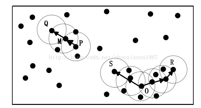
上图为“密度直达”和“密度可达”概念示意描述。根据前文基本概念的描述知道:由于有标记的各点­M、P、O和R的Eps近邻均包含3个以上的点,因此它们都是核对象;M­是从P“密度直达”;而Q则是从­M“密度直达”;基于上述结果,Q是从P“密度可达”;但P从Q无法“密度可达”(非对称)。类似地,S和R从O是“密度可达”的;O、R和S均是“密度相连”(对称)的。 #### (3)DBSCAN密度聚类思想     DBSCAN的聚类定义很简单:由密度可达关系导出的最大密度相连的样本集合,即为我们最终聚类的一个类别,或者说一个簇。

    这个DBSCAN的簇里面可以有一个或者多个核心对象。如果只有一个核心对象,则簇里其他的非核心对象样本都在这个核心对象的ϵ-邻域里;如果有多个核心对象,则簇里的任意一个核心对象的ϵ-邻域中一定有一个其他的核心对象,否则这两个核心对象无法密度可达。这些核心对象的ϵ-邻域里所有的样本的集合组成的一个DBSCAN聚类簇。

    那么怎么才能找到这样的簇样本集合呢?DBSCAN使用的方法很简单,它任意选择一个没有类别的核心对象作为种子,然后找到所有这个核心对象能够密度可达的样本集合,即为一个聚类簇。接着继续选择另一个没有类别的核心对象去寻找密度可达的样本集合,这样就得到另一个聚类簇。一直运行到所有核心对象都有类别为止。

    基本上这就是DBSCAN算法的主要内容了,是不是很简单?但是我们还是有三个问题没有考虑。

    第一个是一些异常样本点或者说少量游离于簇外的样本点,这些点不在任何一个核心对象在周围,在DBSCAN中,我们一般将这些样本点标记为噪音点。

    第二个是距离的度量问题,即如何计算某样本和核心对象样本的距离。在DBSCAN中,一般采用最近邻思想,采用某一种距离度量来衡量样本距离,比如欧式距离。这和KNN分类算法的最近邻思想完全相同。对应少量的样本,寻找最近邻可以直接去计算所有样本的距离,如果样本量较大,则一般采用KD树或者球树来快速的搜索最近邻。如果大家对于最近邻的思想,距离度量,KD树和球树不熟悉,建议参考之前写的另一篇文章K近邻法(KNN)原理小结。

    第三种问题比较特殊,某些样本可能到两个核心对象的距离都小于ϵ,但是这两个核心对象由于不是密度直达,又不属于同一个聚类簇,那么如果界定这个样本的类别呢?一般来说,此时DBSCAN采用先来后到,先进行聚类的类别簇会标记这个样本为它的类别。也就是说DBSCAN的算法不是完全稳定的算法。 #### (4)DBSCAN聚类算法 算法表达一: 输入:样本集\(D=(x_1,x_2,...,x_m)\),邻域参数\((\epsilon,MinPts)\),样本距离度量方式。 输出:簇划分\(C\) 1. 初始化核心对象集合\(\Omega=\emptyset\),初始化聚类簇数\(k=0\),初始化未访问的样本集合\(\Gamma=D\),簇划分\(C=\emptyset\) 2. 对于\(j=1,2,...,m\),按下面的步骤找出所有的核心对象: a)通过距离度量方式,找到样本\(x_j\)\(\epsilon\)-邻域子样本集\(N_\epsilon(x_j)\) b)如果子样本集的样本个数满足\(\vert N_\epsilon(x_j)\vert\ge MinPts\),将样本\(x_j\)加入核心对象样本集合:\(\Omega=\Omega\cup \{x_j\}\) 3. 如果核心对象集合\(\Omega=\emptyset\),则算法结束,否则转入步骤4 4. 在核心对象集合\(\Omega\)中,随机选择一个核心对象\(o\),初始化当前簇核心对象列队\(\Omega_{cur}=\{o\}\),初始化类别序号\(k=k+1\),初始化当前簇样本集合\(C_k=\{o\}\),更新未访问样本集合\(\Gamma=\Gamma-{o}\) 5. 如果当前簇核心对象列队\(\Omega_{cur}\ne\emptyset\),转入步骤6,否则当\(\Omega_{cur}=\emptyset\),则当前聚类簇\(C_k\)生成完毕,更新簇划分\(C=\{C_1,C_2,...,C_k\}\),更新核心对象集合\(\Omega=\Omega-C_k\),转入步骤3 5. 在当前簇核心对象队列\(\Omega_{cur}\)中取出一个核心对象,通过邻域距离阈值\(\epsilon\)找出所有的\(\epsilon\)-邻域子样本集\(N_\epsilon(o^\prime)\),令\(\Delta=N_\epsilon(o^\prime)\cap\Gamma\),更新当前簇样本集合\(C_k=C_k\cup \Delta\),更新未访问样本集合\(\Gamma=\Gamma-\Delta\),更新\(\Omega_{cur}=\Omega_{cur}\cup(\Delta\cap\Omega)-o^\prime\),转入步骤5

输出结果为:簇划分\(C=\{C_1,C_2,...,C_k\}\)

算法表达二输入\(D\):一个包含\(n\)个对象的数据集 \(\epsilon\):半径参数 \(MinPts\):邻域密度阈值 输出:基于密度的簇的集合 步骤: 1. 标记所有对象为unvisited 2. Do 3. 随机选择一个unvisited对象\(p\) 4. 标记\(p\)visited 5. If \(p\)\(\epsilon\)-邻域至少有\(MinPts\)个对象 6.   创建一个新簇\(C\),并把\(p\)添加到\(C\) 7.   令\(N\)\(p\)\(\epsilon\)-邻域中的对象集合 8.   For \(N\) 中的每个点\(q\) 9.     If \(q\)是unvisited 10.       标记\(q\)为visited 11.       If \(q\)\(\epsilon\)-邻域至少有\(MinPts\)个对象,把这些对象添加到\(N\) 12.       If \(q\)还不是任何簇的成员,把\(q\)添加到\(C\) 13.  End for 14.  输出\(C\) 15. Else标记\(p\)为噪声 16. Until没有标记为unvisited的对象

(5)DBSCAN小结

    和传统的K-Means算法相比,DBSCAN最大的不同就是不需要输入类别数k,当然它最大的优势是可以发现任意形状的聚类簇,而不是像K-Means,一般仅仅使用于凸的样本集聚类。同时它在聚类的同时还可以找出异常点,这点和BIRCH算法类似。

    那么我们什么时候需要用DBSCAN来聚类呢?一般来说,如果数据集是稠密的,并且数据集不是凸的,那么用DBSCAN会比K-Means聚类效果好很多。如果数据集不是稠密的,则不推荐用DBSCAN来聚类。

    下面对DBSCAN算法的优缺点做一个总结。

    DBSCAN的主要优点有:

    1) 可以对任意形状的稠密数据集进行聚类,相对的,K-Means之类的聚类算法一般只适用于凸数据集。

    2) 可以在聚类的同时发现异常点,对数据集中的异常点不敏感。

    3) 聚类结果没有偏倚,相对的,K-Means之类的聚类算法初始值对聚类结果有很大影响。

    DBSCAN的主要缺点有:

    1)如果样本集的密度不均匀、聚类间距差相差很大时,聚类质量较差,这时用DBSCAN聚类一般不适合。

    2) 如果样本集较大时,聚类收敛时间较长,此时可以对搜索最近邻时建立的KD树或者球树进行规模限制来改进。

    3) 调参相对于传统的K-Means之类的聚类算法稍复杂,主要需要对距离阈值ϵ,邻域样本数阈值MinPts联合调参,不同的参数组合对最后的聚类效果有较大影响。

1.利用百度地图得到行政区域轮廓线

利用到的API函数:Boundary()

代码实例:

1
2
3
4
5
6
7
8
9
10
11
12
13
14
15
16
17
18
19
20
21
22
23
24
25
26
27
28
29
30
31
32
33
34
35
36
37
38
39
40
41
<!DOCTYPE html PUBLIC "-//W3C//DTD XHTML 1.0 Transitional//EN" "http://www.w3.org/TR/xhtml1/DTD/xhtml1-transitional.dtd">
<html xmlns="http://www.w3.org/1999/xhtml">
<head>
<meta http-equiv="Content-Type" content="text/html; charset=utf-8" />
<title>获取地区轮廓线</title>
<script type="text/javascript" src="http://api.map.baidu.com/api?v=1.3">
</script>
<style type="text/css">
body{font-size:13px;margin:10px}
#container{width:800px;height:500px;border:1px solid gray;margin:auto auto;}
#controler {text-align:center;margin-top:30px;}
</style>
</head>
<body>
<div id="container"></div>
<div id="controler">
输入省、直辖市或县名称:<input type="text" id="districtName" style="width:80px" value="合肥市">
<input type="button" onclick="getBoundary()" value="获取轮廓线"></div>

<script type="text/javascript">
var map = new BMap.Map("container");
map.centerAndZoom(new BMap.Point(116.403765, 39.914850), 5);
map.addControl(new BMap.NavigationControl({type: BMAP_NAVIGATION_CONTROL_SMALL}));
map.enableScrollWheelZoom();

function getBoundary(){
var bdary = new BMap.Boundary();
var name = document.getElementById("districtName").value;
bdary.get(name, function(rs){ //获取行政区域
map.clearOverlays(); //清除地图覆盖物
var count = rs.boundaries.length; //行政区域的点有多少个
for(var i = 0; i < count; i++){
var ply = new BMap.Polygon(rs.boundaries[i], {strokeWeight: 2, strokeColor: "#ff0000"}); //建立多边形覆盖物
map.addOverlay(ply); //添加覆盖物
map.setViewport(ply.getPath()); //调整视野
}
});
}
</script>
</body>
</html>

显示效果为

2.接下来是根据坐标获取位置的行政区信息

API信息: http://lbsyun.baidu.com/index.php?title=webapi/guide/webservice-geocoding-abroad

1
http://api.map.baidu.com/geocoder/v2/?callback=renderReverse&location=35.658651,139.745415&output=json&pois=1&ak=您的ak //GET请求
主要是更改location这个变量,这里有个问题,返回的数据格式不是严格的json格式字符串:
1
renderReverse&&renderReverse({"status":0,"result":{"location":{"lng":116.33815299999995,"lat":39.94171507488761},"formatted_address":"北京市海淀区新苑街13号","business":"白石桥,车公庄,甘家口","addressComponent":{"country":"中国","country_code":0,"country_code_iso":"CHN","country_code_iso2":"CN","province":"北京市","city":"北京市","city_level":2,"district":"海淀区","town":"","adcode":"110108","street":"新苑街","street_number":"13号","direction":"附近","distance":"16"},"pois":[{"addr":"北京市海淀区三里河路1号11号楼(西苑饭店院内)","cp":" ","direction":"东南","distance":"129","name":"中国外贸金融租赁","poiType":"金融","point":{"x":116.3375433561377,"y":39.94247976148231},"tag":"金融;投资理财","tel":"","uid":"7c6d3881a8f4e35c1d5800e7","zip":"","parent_poi":{"name":"","tag":"","addr":"","point":{"x":0.0,"y":0.0},"direction":"","distance":"","uid":""}},{"addr":"三里河路5号","cp":" ","direction":"西北","distance":"105","name":"五矿发展大厦-C座","poiType":"房地产","point":{"x":116.33879200079658,"y":39.94117976632641},"tag":"房地产;写字楼","tel":"","uid":"db101a6a677f6af9c7f02567","zip":"","parent_poi":{"name":"五矿发展大厦","tag":"房地产;写字楼","addr":"北京市海淀区三里河路7号","point":{"x":116.33929505188216,"y":39.94086859358035},"direction":"西北","distance":"176","uid":"d97e2bb301449ac60b1cc703"}},{"addr":"北京市海淀区三里河路1号","cp":" ","direction":"南","distance":"225","name":"西苑饭店","poiType":"酒店","point":{"x":116.33881894996186,"y":39.943185067585059},"tag":"酒店;五星级","tel":"","uid":"eb3675036510d10201ec0197","zip":"","parent_poi":{"name":"","tag":"","addr":"","point":{"x":0.0,"y":0.0},"direction":"","distance":"","uid":""}},{"addr":"北京市海淀区三里河5号","cp":" ","direction":"西","distance":"126","name":"五矿发展大厦-B座","poiType":"房地产","point":{"x":116.33926810271686,"y":39.941553171738828},"tag":"房地产;写字楼","tel":"","uid":"a12baa40e1bdd956e956faae","zip":"","parent_poi":{"name":"五矿发展大厦","tag":"房地产;写字楼","addr":"北京市海淀区三里河路7号","point":{"x":116.33929505188216,"y":39.94086859358035},"direction":"西北","distance":"176","uid":"d97e2bb301449ac60b1cc703"}},{"addr":"北京市海淀区三里河路7号","cp":" ","direction":"西北","distance":"176","name":"五矿发展大厦","poiType":"房地产","point":{"x":116.33929505188216,"y":39.94086859358035},"tag":"房地产;写字楼","tel":"","uid":"d97e2bb301449ac60b1cc703","zip":"","parent_poi":{"name":"","tag":"","addr":"","point":{"x":0.0,"y":0.0},"direction":"","distance":"","uid":""}},{"addr":"北京市海淀区西苑饭店南门","cp":" ","direction":"东南","distance":"119","name":"新苑街-15号院","poiType":"房地产","point":{"x":116.3375164069724,"y":39.94238295419036},"tag":"房地产;住宅区","tel":"","uid":"da5b62ec876c0e3b725e8089","zip":"","parent_poi":{"name":"","tag":"","addr":"","point":{"x":0.0,"y":0.0},"direction":"","distance":"","uid":""}},{"addr":"海淀区三里河路甲1号西苑饭店副楼(动物园地铁站向西300米)","cp":" ","direction":"南","distance":"196","name":"养怡园食府","poiType":"美食","point":{"x":116.33805539027839,"y":39.943074431818278},"tag":"美食;中餐厅","tel":"","uid":"4ce10ce6608cf0b8441a321b","zip":"","parent_poi":{"name":"","tag":"","addr":"","point":{"x":0.0,"y":0.0},"direction":"","distance":"","uid":""}},{"addr":"北京市海淀区三里河路5号","cp":" ","direction":"东北","distance":"214","name":"五色土幼儿园","poiType":"教育培训","point":{"x":116.3371301356031,"y":39.940460609374458},"tag":"教育培训;幼儿园","tel":"","uid":"d6ee87244bf557e0a8f0cd7d","zip":"","parent_poi":{"name":"","tag":"","addr":"","point":{"x":0.0,"y":0.0},"direction":"","distance":"","uid":""}},{"addr":"三里河路7号","cp":" ","direction":"北","distance":"293","name":"北京国玉新疆和田玉文博馆","poiType":"购物","point":{"x":116.33848657692318,"y":39.93969995430771},"tag":"购物;商铺","tel":"","uid":"a662490a8097cd8adeee8b02","zip":"","parent_poi":{"name":"新疆大厦","tag":"酒店;其他","addr":"三里河路7号","point":{"x":116.33838776331707,"y":39.93911908469923},"direction":"北","distance":"376","uid":"50fb64fffbeb6f44e8f853ed"}},{"addr":"三里河路7号(北京西苑饭店南150米处)","cp":" ","direction":"北","distance":"314","name":"北京新疆大厦嘉宾楼","poiType":"酒店","point":{"x":116.33879200079658,"y":39.93959622795643},"tag":"酒店;其他","tel":"","uid":"dba22815e682addc4afd3ff8","zip":"","parent_poi":{"name":"新疆大厦","tag":"酒店;其他","addr":"三里河路7号","point":{"x":116.33838776331707,"y":39.93911908469923},"direction":"北","distance":"376","uid":"50fb64fffbeb6f44e8f853ed"}}],"roads":[],"poiRegions":[],"sematic_description":"中国外贸金融租赁东南129米","cityCode":131}})
因此需要正则表达式来进行提取:
1
r=re.findall(r"[(](.*)[)]$",response.text)##text里面为返回的字符串
同时,返回的数据是Unicode格式,json模块无法解析,因而需要先对其进行转码:
1
2
res=r[0].encode("utf-8")
rj=json.loads(res)
这里附加关于json模块的相关信息: 1. json.dumps()和json.loads()是json格式处理函数(可以这么理解,json是字符串)   (1)json.dumps()函数是将一个Python数据类型列表进行json格式的编码(可以这么理解,json.dumps()函数是将字典转化为字符串)   (2)json.loads()函数是将json格式数据转换为字典(可以这么理解,json.loads()函数是将字符串转化为字典)

  1. json.dump()和json.load()主要用来读写json文件函数